Dynamic Path Planning of a Mobile Robot
with Improved Q-Learning Algorithm

S. Li, X. Xu and L. Zuo,
Dynamic path planning of a mobile robot
with improved Q-learning algorithm,
IEEE International Conference on
Information and Automation, 2015

Exam Presentation
Learning for Autonomous Systems Course
SDIC Master Degree, University of Trieste (UniTS)

Marco Tallone
June 2025

Table of Contents

  1. MDP OF PATH PLANNING PROBLEM
  2. EXPLORATION STRATEGIES AND HEURISTICS
  3. IMPROVED Q-LEARNING ALGORITHM
  4. SIMULATION AND ANALYSIS

OBJECTIVE

Present a novel approach to path planning for mobile robots using an improved Q-learning algorithm, with alternative exploration strategy and heuristics to reduce the search space and improve performance

Markov Decision Problem Model
of Path Planning Problem

Markov Decision Process (MDP)

$\mathcal{S}$ : finite set of states ($|\mathcal{S}| = n$)
$\mathcal{A}$ : finite set of actions ($|\mathcal{A}| = m$)
\[ P: \mathcal{S} \times \mathcal{A} \times \mathcal{S} \to [0, 1] \] transition probability function
\[ R: \mathcal{S} \times \mathcal{A} \times \mathcal{S} \to \mathbb{R} \] reward function

The expected reward for taking action $a_k$ in state $s_k$ at time $k$ and transitioning to $s_{k+1}$ is: \[ r_{k+1} = \sum_{s_{k+1} \in \mathcal{S}} P(s_{k+1} | s_k, a_k) R(s_k, a_k, s_{k+1}) \tag{1} \]

Markov Decision Process (MDP)

MDP Problem Objective:
$\rightarrow$ find optimal policy $\pi^*$ maximizing the expected discounted cumulative reward:

\[ \pi^* = \arg\max_{\pi} \mathbb{E}\left[\sum_{k=0}^{\infty} \gamma^k r_k\right] \]

where $\gamma \in [0, 1[$ is the discount factor which weights rewards over time,
while $\pi : \mathcal{S} \to \mathcal{A}$ is the policy that maps states to actions: $\pi(s_k) = a_k$

Path Planning Problem

Formal definition of the Path Planning Problem:

Path Planning Problem
Find out an optimal, collision-free path from an initial point $s_0$ to a target point $s_g$

  • optimal $\rightarrow$ given a chosen set of criterias
    such as shortest path, minimum energy consumption, minimum time, etc.
    Here, the optimality criteria is defined as the shortest path from state $s_0$ to the goal $s_g$
  • collision-free $\rightarrow$ the path must not intersect with any obstacle in the environment

Environment Model and States

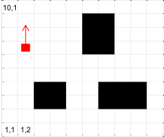
A grid-based model represents the environment space

Assume there are:

  • static indeterminate obstacles (⬛)
  • moving obstacles (🟥):
    constant orientation and speed

States: cells of the grid, i.e. pairs of coordinates $(x, y)$
(E.g. $(1,1), (1,2), \dots, (10,1), \dots$)
Grid-based Environment Model

Actions

Actions:
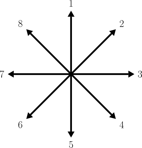
Set of $8$ possible oriented movements inside the grid:

  1. up $\uparrow$
  2. right-up $\nearrow$
  3. right $\rightarrow$
  4. right-down $\searrow$
  5. down $\downarrow$
  6. left-down $\swarrow$
  7. left $\leftarrow$
  8. left-up $\nwarrow$
The 8 actions

Reward Function

To affect agent learning to move towards the goal, we define the following reward function:

\[ R(s_k, a_k, s_{k+1}) = \alpha \cdot (d_{s_k} - d_{s_{k+1}}) - \beta \cdot \frac{1}{d_o} \tag{3} \]

where:

  • $d_{s_k}$: distance of the current state $s_k$ to the goal state
  • $d_{s_{k+1}}$: distance of the next state $s_{k+1}$ to the goal state
  • $d_o$: distance of next state $s_{k+1}$ to the closest obstacle
  • $\alpha, \beta$: constant weighting parameters

Action-Value Function

The Action-Value Function $Q_{\pi}(s_k, a_k)$ describes the quality of transitions from state $s_k$ to the next, by immediately taking action $a_k$ and then following policy $\pi$.

The exact $Q_{\pi}$ values for all state-action pairs can be computed using the Bellman equation: \[ Q_{\pi}(s_k, a_k) = r_{k+1} + \gamma \sum_{s_{k+1} \in \mathcal{S}} P(s_{k+1} | s_k, a_k) \sum_{a_{k+1} \in \mathcal{A}} Q_{\pi}(s_{k+1}, a_{k+1}) \tag{2} \]

The optimal control policy $\pi^*$ can be obtained from the optimal action-value function $Q^*$: \[ \pi^*(s_k) = \arg\max_{a_k} Q^*(s_k, a_k) \]

⚠️ Note: In the model-free case we don't know the transition probabilities $P$

$Q$-Learning

$Q$-Learning is a model-free approach that be used to find the optimal action policy $\pi^*$

In the "learning phase", the agent explores the environment and learns the $Q$-values for all state-action pairs $(s_k, a_k)$ by iteratively updating the $Q$-table based on a greedy approach (off-policy):

\[ Q(s_k, a_k) \leftarrow Q(s_k, a_k) + \alpha \cdot \left[ r_{k+1} + \gamma \cdot \max_{a} Q(s_{k+1}, a) - Q(s_k, a_k) \right] \tag{6} \]

Assuming $n$ states and $m$ actions, the $Q$-table is a matrix of size $n \times m$

$Q$-learning is based on an episodic approach, where each episode ends when the agent reaches the goal state $s_g$ or an obstacle state $s_o$

$Q$-Learning Algorithm Example

Simple $1 \times 6$ grid environment with a goal state $s_g = 5$ and an obstacle at $s_o = 0$

\[ \mathcal{S} = \{0, 1, 2, 3, 4, 5\} \quad \quad \quad \quad \mathcal{A} = \{-1, +1\} \]

Assuming $\alpha = 1$ and $\gamma = 1$, simplifies the update to: \[ Q(s_k, a_k) \leftarrow r_{k+1} + \max_{a} Q(s_{k+1}, a) \]

Where reward $r_{k+1}$ is defined as: \[ r_{k+1} = (d_{s_k} - d_{s_{k+1}}) - \frac{1}{d_o} \]

Q-Learning Algorithm - Example
$Q$-table $-1$ ($\leftarrow$) $+1$ ($\rightarrow$)
$0$ $0$ $0$
$1$ $0$ $0$
$2$ $0$ $0$
$3$ $0$ $0$
$4$ $0$ $0$
$5$ $0$ $0$

$Q$-Learning Algorithm Example

Episode $1$:

  • Randomly select initial state $s_0 = 2$
  • Randomly select action $a_0 = +1 (\rightarrow)$

Episode time-steps:

  1. $s_1 = 3$, $r_1 = (3-2) - \frac{1}{3} = 0.67$ $\Rightarrow$ $Q(2, +1) = 0.67$
  2. $s_2 = 4$, $r_2 = (2-1) - \frac{1}{4} = 0.75$ $\Rightarrow$ $Q(3, +1) = 0.75$
  3. $s_3 = 5$, $r_3 = (1-0) - \frac{1}{5} = 0.8$ $\Rightarrow$ $Q(4, +1) = 0.8$
    ✅ TERMINAL CONDITION $s_3 = s_g = 5$

Q-Learning Algorithm - Example
$Q$-table $-1$ ($\leftarrow$) $+1$ ($\rightarrow$)
$0$ $0$ $0$
$1$ $0$ $0$
$2$ $0$ $0.67$
$3$ $0$ $0.75$
$4$ $0$ $0.8$
$5$ $0$ $0$

$Q$-Learning Algorithm Example

Episode $2$:

  • Randomly select initial state $s_0 = 2$
  • Randomly select action $a_0 = -1 (\leftarrow)$

Episode time-steps:

  1. $s_1 = 1$, $r_1 = (3-4) - \frac{1}{1} = -2 $ $\Rightarrow$ $Q(2, +1) = -2$
  2. $s_2 = 0$, $r_2 = (4-5) - \frac{1}{0} = -\infty$ $\Rightarrow$ $Q(1, -1) = -\infty$
    ❌ TERMINAL CONDITION $s_2 = s_o = 0$ (obstacle)


Episode $3$: $\dots$

After enough episodes, the agent learns the optimal $Q$-table for all state-action pairs $\dots$

Q-Learning Algorithm - Example
$Q$-table $-1$ ($\leftarrow$) $+1$ ($\rightarrow$)
$0$ $0$ $0$
$1$ $- \infty$ $0$
$2$ $-2$ $0.67$
$3$ $0$ $0.75$
$4$ $0$ $0.8$
$5$ $0$ $0$

Exploration Strategies and Heuristics

Exploration - Exploitation Trade-off

In Reinforcement Learning techniques such as $Q$-Learning we need to balance:

  • Exploration: trying new actions $a_k$ to possibly discover better Strategies
  • Exploitation: using the current knowledge to maximize the expected reward

The performance of the $Q$-Learning algorithms is affected by the exploration strategy used

Two possible exploration strategies are:

ε-Greedy
Boltzmann

ε-Greedy Exploration

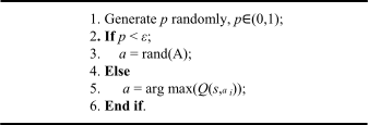
In most cases, it takes a greedy approach and chooses the best action $a_k$ according to the current $Q$-values (exploitation), but with a small probability $\varepsilon$ it chooses a random action instead (exploration).

ε-Greedy Exploration Algorithm

Boltzmann Exploration

At the beginning of the learning, the probability of the random action is larger than the probability of the greedy action, but as the learning progresses, the probability $p$ of the greedy action increases.
The agent selects the best action $a_i$ with probability $p$ computed as:

\[ p(s, a_i) = \frac{e^{Q(s, a_i) / T}}{\sum_{a_k \in \mathcal{A}} e^{Q(s, a_k) / T}} \tag{4} \] with: \[ T_k = \lambda^k T_0 \tag{5} \] where $\lambda \in [0, 1[$ is a temperature discount rate.

New Exploration strategy

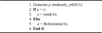
A new exploration strategy is proposed, which combines the ε-Greedy strategy with probability $\varepsilon$ and Boltzmann strategy with complementary $1 - \varepsilon$ probability.

ε-Greedy Exploration Algorithm

When ε-Greedy is not selected, we still allow exploration through the Boltzmann strategy, but converging to the greedy approach as the temperature decreases.
$\Rightarrow$ avoids local optimum and accelerates the expected $Q$-values convergence to optimality

Heuristic Searching Strategies

$Q$-Learning easily suffers from the curse of dimensionality when the state space $\mathcal{S}$ and the action space $\mathcal{A}$ are large ($n \gg 1$ and $m \gg 1$)

To reduce the search space, we can use heuristic searching strategies that must be satisfied when selecting random actions in exploration strategies. Given current state $s_k=(x_k, y_k)$:

  • If $(x_k < x_g) \land (y_k < y_g)$ $\Rightarrow$ $a_{k+1} = \text{rand}(1, 2, 3)$
    else if $(x_k > x_g) \land (y_k > y_g)$ $\Rightarrow$ $a_{k+1} = \text{rand}(5, 6, 7)$
  • If $(x_k < x_g) \land (y_k > y_g)$ $\Rightarrow$ $a_{k+1} = \text{rand}(3, 4, 5)$
    else if $(x_k > x_g) \land (y_k < y_g)$ $\Rightarrow$ $a_{k+1} = \text{rand}(7, 8, 1)$
  • If $(x_k = x_g) \lor (y_k = y_g)$ $\Rightarrow$ $a_{k+1} = \text{rand}(1,5) \lor \text{rand}(3,7)$
  • Else $a_{k+1} = \text{rand}\{a_{k} - 1, a_{k}, a_{k} + 1\}$
    (limits the variation range within $0^{\circ} - 90^{\circ}$)

The 8 actions

Improved Q-Learning Algorithm

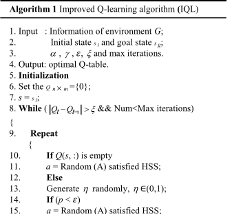
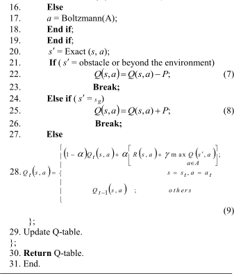
Improved $\;Q$-Learning (IQL) Algorithm

Improved Q-Learning Algorithm - Top
Improved Q-Learning Algorithm - Bottom

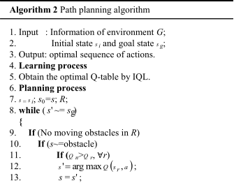
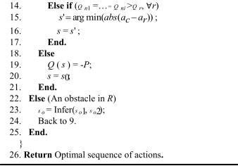
Path Planning Algorithm

Improved Q-Learning Algorithm - Top
Improved Q-Learning Algorithm - Bottom

Simulation and Analysis

Methodology

  1. Obtain the optimal $Q$-table using the Improved $Q$-Learning (IQL)
    algorithm in a static environment with static obstacles
  2. Apply the obtained $Q$-table to different dynamic environments
    with both moving and static obstacles

Consider grid environment with $20 \times 20$ cells, hence:
  • $n = 400$ states
  • $m = 8$ actions

Static Environment

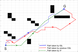
Static Environment 1

Fig. 3: Environment with static obstacles known a priori

Unknown Static Environment

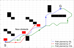
Static Environment 2

Fig. 4: Environment with static obstacles not known a priori

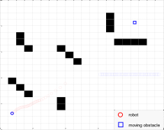
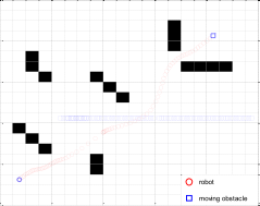
Dynamic Environment

Dynamic Environment 1 Dynamic Environment 2 Dynamic Environment 3

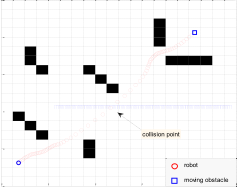
Fig. 5: Environment with moving obstacles

Random Initial Point

Random Initial Point

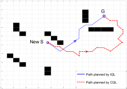
Fig. 6: Environment with random initial point

Execution Time Comparison

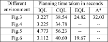
Comparison of the execution times in diferent methods
"--" means that the method failed to plan the path

Time Comparison